使用 kallisto 可以对原始 RNA-seq 数据的 Reads 结果进行分析,统计每一基因的 counts 估计值、 TPM 值等对寻找差异表达基因有用的值, kallisto 是基于 pseudoalignment 的算法,能够快速分析二代测序结果,而其结果的分析与解读工具又可以使用相应的 R 包来完成,就是 Sleuth,不过这个包还再开发完善中,并未发表相关的文章,鉴于是针对 Kallisto 的下游分析工具,可以先来尝试一下
Sleuth 包的安装
- Sleuth 包还没有发布,所以只能通过 github 来安装,先安装
rhdf5再安装devtools最后通过 github 安装sleuth - 安装:
>source("http://bioconductor.org/biocLite.R")
>biocLite("rhdf5")
>install.packages("devtools")
>devtools::install_github("pachterlab/sleuth")
数据导入
- sleuth 是基于 kallisto 结果的后续分析,所以可以直接读取 kallisto 输出的结果
abundance.h5文件或者abundance.tsv文件 - abundance.tsv 结果如下:
        target_id length eff_length est_counts tpm
1 ENST00000415118      8     5.0000          0   0
2 ENST00000448914     13    10.0000          0   0
3 ENST00000434970      9     6.0000          0   0
4 ENST00000390577     37    10.0625          0   0
5 ENST00000437320     19    16.0000          0   0
6 ENST00000450276     17    14.0000          0   0
- 下载Sleuth测试数据进行测试,放在
~/sample/kallisto/test/下
>library("sleuth")
>base_dir <- "~/sample/kallisto/test/"
>sample_id <- dir(file.path(base_dir,"results"))
>kal_dirs <- sapply(sample_id, function(id) file.path(base_dir, "results", id, "kallisto"))
>s2c <- read.table(file.path(base_dir, "hiseq_info.txt"), header = TRUE, stringsAsFactors=FALSE)
>s2c <- dplyr::select(s2c, sample = run_accession, condition)
>s2c <- dplyr::mutate(s2c, path = kal_dirs)
>so <- sleuth_prep(s2c, ~ condition)
reading in kallisto results
......
normalizing est_counts
50844 targets passed the filter
normalizing tpm
merging in metadata
normalizing bootstrap samples
summarizing bootstraps
分析及结果输出
>so <- sleuth_fit(so)
>so <- sleuth_wt(so, which_beta = 'conditionscramble')
>results_table <- sleuth_results(so, 'conditionscramble')
>write.csv(results_table,"results_test.csv")
> head(results_table)
        target_id pval qval          b       se_b mean_obs   var_obs
1 ENST00000075120    0    0 -1.4661181 0.03535490 7.910524 0.6463507
2 ENST00000244745    0    0 -1.6483482 0.04193705 7.568028 0.8172260
3 ENST00000249749    0    0 -2.6770431 0.06291763 6.452782 2.1533039
4 ENST00000256646    0    0  0.9454387 0.02496143 8.218254 0.2688586
5 ENST00000257497    0    0  1.0245592 0.02474028 8.313881 0.3156510
6 ENST00000263734    0    0  1.3233153 0.02526430 8.213073 0.5255182
      tech_var      sigma_sq smooth_sigma_sq final_sigma_sq
1 0.0006033334  1.271621e-03    0.0006840236   0.0012716205
2 0.0007067384  1.931335e-03    0.0007652357   0.0019313352
3 0.0042122927 -4.232682e-05    0.0017256493   0.0017256493
4 0.0002716565  6.062440e-04    0.0006629529   0.0006629529
5 0.0002418629  6.762591e-04    0.0006657409   0.0006762591
6 0.0002944993 -8.305197e-05    0.0006629280   0.0006629280
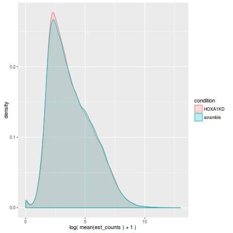
组间 counts 密度图
>plot_group_density(so)
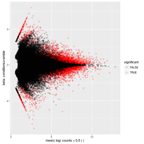
MA 图
>plot_ma(so,test='conditionscramble')
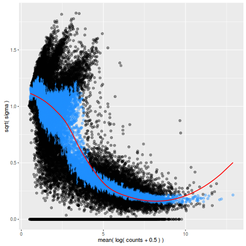
均值-方差分析
>plot_mean_var(so)
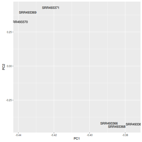
PCA分析
>plot_pca(so,text_labels=TRUE)
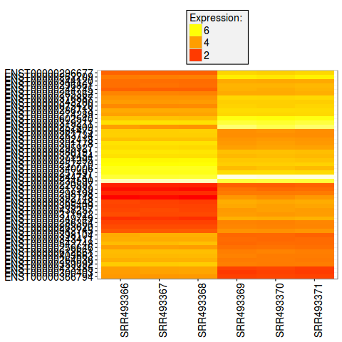
heatmap(top50) 图
>library(pheatmap)
>plot_transcript_heatmap(so,transcripts = results_table$target_id[1:50])
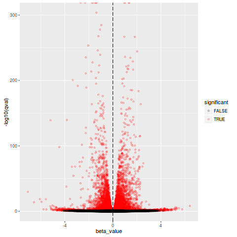
火山图
>plot_volcano(so,test="conditionscramble")